We are now able to give the proof of the following weak form of the straightening algorithm.
 mod
mod PROOF: We divide into the following two cases
Case 1:
By assumption there are two consecutive indices ![]() and
and ![]() in
in
![]() such that
such that
![]() and
and
![]() . If
. If
![]() , we have
, we have
![]() by Corollary 9.2, implying our assertion.
In the case
by Corollary 9.2, implying our assertion.
In the case
![]() we apply Corollary 9.12:
we apply Corollary 9.12:
The multi-indices ![]() in the sum satisfy
in the sum satisfy
![]() and consequently
and consequently
![]() . Finally, since
. Finally, since
![]() and
and
![]() occurs before
occurs before ![]() in the
lexicographic order on
in the
lexicographic order on ![]() we have
we have
![]() as well.
as well.
Case 2:
In principle we follow the lines of the proof of [Ma, 2.5.7].
But since
![]() is not commutative we have to
work with a fixed basic tableau. The change of
basic tableaux in [Ma, 2.5.7] can be compensated for by
Lemma 9.8.
is not commutative we have to
work with a fixed basic tableau. The change of
basic tableaux in [Ma, 2.5.7] can be compensated for by
Lemma 9.8.
To start, let
![]() be the
smallest index such that
be the
smallest index such that ![]() is larger than its right hand neighbour
is larger than its right hand neighbour
![]() in the
in the ![]() -tableau of
-tableau of ![]() .
Assume that the entry
.
Assume that the entry ![]() lies in the
lies in the ![]() -th column
-th column
![]() and that
and that ![]() lies in the
lies in the ![]() -th column
-th column
![]() ,
where
,
where
![]() . Clearly,
. Clearly,
![]() .
Let
.
Let ![]() be the index of the row containing both entries. We picture this
by
be the index of the row containing both entries. We picture this
by
By assumption we have
![]() . Now, we refine the dual partition
. Now, we refine the dual partition
![]() of
of ![]() to a
composition
to a
composition
![]() , where
, where
![]() is the number of columns of the diagram of
is the number of columns of the diagram of ![]() . More
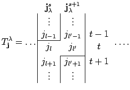
precisely, we split the
. More
precisely, we split the
![]() -th and
-th and ![]() -th column in front of and below the
-th column in front of and below the ![]() -th row:
-th row:
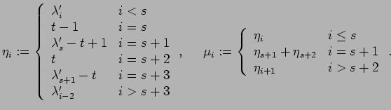
Obviously, this ![]() is the coarsest refinement of the partition
is the coarsest refinement of the partition ![]() and the composition
and the composition
![]() defined above. Let us split the multi-index
defined above. Let us split the multi-index ![]() according to
according to ![]() as follows:
as follows:
Here,
![]() is the index of the
first entry of the
is the index of the
first entry of the ![]() -th column and
-th column and
![]() (resp.
(resp.
![]() ) are the lengths of both columns in question.
We have
) are the lengths of both columns in question.
We have
In order to apply Laplace Duality 9.7 to the pair
![]() of compositions
we have to choose coset representatives of
of compositions
we have to choose coset representatives of
![]() in
in
![]() and
and
![]() carefully. From the theory of
parabolic subgroups of reflection groups it is known that each right coset
of
carefully. From the theory of
parabolic subgroups of reflection groups it is known that each right coset
of
![]() in
in
![]() contains a unique element of minimal length called the distinguished
right coset representative, in fact one looks for coset representatives of
contains a unique element of minimal length called the distinguished
right coset representative, in fact one looks for coset representatives of
![]() in
in
![]() . We choose these for our set
. We choose these for our set ![]() . The property
. The property
![]() for
for ![]() and
and
![]() follows from
that theory as well. Similarily, one finds a set
follows from
that theory as well. Similarily, one finds a set ![]() of distinguished
left coset representatives of
of distinguished
left coset representatives of
![]() in
in
![]() satisfying
satisfying
![]() for
for
![]() and
and ![]() .
.
We will not apply Laplace Duality to the original index pair
![]() , for we must handle the transition from the
order
, for we must handle the transition from the
order ![]() to
to ![]() . Instead of
. Instead of ![]() we rather consider
we rather consider
![]() where
where
![]() is chosen in such a way
that
is chosen in such a way
that
![]() and
and ![]() for
for
![]() and
and
![]() (the embedding of
(the embedding of
![]() is
understood according to the composition
is
understood according to the composition ![]() ). This
). This ![]() exists uniquely
since
exists uniquely
since
![]() contains exactly
contains exactly
![]() elements by the assumption
elements by the assumption
![]() on
on ![]() .
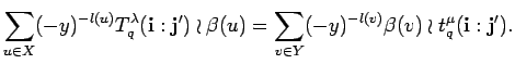
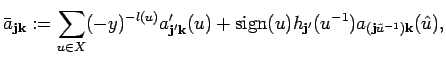
Now, by Laplace-Duality we obtain
.
Now, by Laplace-Duality we obtain
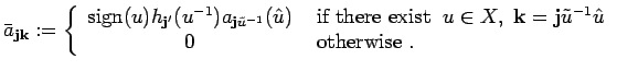
With help of Lemma 9.8 the right hand side of this equation
can be written as a linear combination of
bideterminants
![]() . Thus the right hand side
is seen to lie in
. Thus the right hand side
is seen to lie in
![]() as soon we have shown that
as soon we have shown that
![]() . But that follows since the longest column
being removed from the diagram of
. But that follows since the longest column
being removed from the diagram of ![]() to obtain the diagram of
to obtain the diagram of ![]() has length
has length
![]() , whereas a column of length
, whereas a column of length
![]() has to be added to the diagram of
has to be added to the diagram of ![]() . On the left hand side of
(12) we may apply Corollary 9.14 by construction
of the multi-index
. On the left hand side of
(12) we may apply Corollary 9.14 by construction
of the multi-index ![]() :
:
the sum running over all ![]() satisfying
satisfying
![]() .
Now, for all
.
Now, for all ![]() we have
we have
![]() since
since
![]() lies in
lies in
![]() . Furthermore, there is a unique
coset representative
. Furthermore, there is a unique
coset representative ![]() satisfying
satisfying
![]() and this is the only one for
which the corresponding
and this is the only one for
which the corresponding
![]() lies in
lies in
![]() . Therefore, in the case
. Therefore, in the case
![]() there is an
there is an ![]() such that
such that
![]() and
and
![]() .
Choose such an
.
Choose such an ![]() for each
for each ![]() . In doing so, we are assigning a
transposition
. In doing so, we are assigning a
transposition
![]() to each
to each ![]() that is contained
in
that is contained
in
![]() . In the case of
. In the case of ![]() we set
we set
![]() .
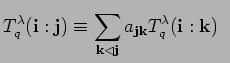
Applying Corollary 9.12 to
.
Applying Corollary 9.12 to ![]() one calculates
one calculates
where the sum runs over all ![]() satisfying
satisfying
![]() , again. For these
, again. For these ![]() we set
we set
whereas in the case
![]() we write
we write
Observe that
![]() occurs in the latter
definition for
occurs in the latter
definition for ![]() .
We assert that for
.
We assert that for ![]() , the multi-index
, the multi-index
![]() occurs before
occurs before ![]() in the
lexicographic order with respect to
in the
lexicographic order with respect to ![]() .
For by construction of
.
For by construction of ![]() and
and ![]() we have
we have
and consequently
![]() . But this implies
. But this implies
![]() ,
since
,
since ![]() for
for ![]() . Thus we obtain
. Thus we obtain
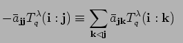 mod
mod
Since the coefficient
![]() is invertible,
the asserted congruence relation holds as well.
is invertible,
the asserted congruence relation holds as well.
![]()
It should be remarked that the proof works with any other
order on
![]() instead of
instead of ![]() , as well. The proof of the
strong part of the algorithm (Proposition 8.3)
can be given right now in the (initial)
case
, as well. The proof of the
strong part of the algorithm (Proposition 8.3)
can be given right now in the (initial)
case ![]() and we are going to do this not only because it is
very instructive, but also because we will need a basis of
and we are going to do this not only because it is
very instructive, but also because we will need a basis of
![]() in order to proceed to the general case.
in order to proceed to the general case.
If ![]() there are exactly two partitions in
there are exactly two partitions in
![]() for
for ![]() ,
namely
,
namely ![]() and
and ![]() , where
, where
![]() and
and
![]() are the fundamental weights (see section 3).
In the first case we have
are the fundamental weights (see section 3).
In the first case we have
![]() , that is, the weak and the strong
form of the straightening algorithm coincide. Turning to
, that is, the weak and the strong
form of the straightening algorithm coincide. Turning to ![]() there is exactly
one element in
there is exactly
one element in
![]() ,
namely
,
namely
![]() .
By (4.3) we obtain in
.
By (4.3) we obtain in
![]()

yielding Proposition 8.3 in the case ![]() since
since
![]() for all
for all ![]() .
.